How to detect credit card fraudsters
This is a pretty long tutorial and I know how hard it is to go through everything, hopefully you may skip a few blocks of code if you need
One of the oldest problem in Statistics is to deal with unbalanced data, for example, surviving data, credit risk, fraud.
Basically, in any data where either your success rate is too high or too low, models are almost irrelevant. This comes from the fact that we use a criteria around 1% to measure the accuracy of a model, ie, if my model predicts in the testing set 99% of the success (or failure depending on what you are trying to do), the model is a hero.

What happens with unbalanced data is that the success metric happening in around 1% (usually less than 10%), so if you have no model and predicts success at 1%, then the model passes the accuracy criteria.
In this post you will learn a ‘trick’ to deal with this type of data: oversampling. In this project I will skip the descriptive analysis hoping that we all want to focus on fraud analysis a bit more.
Importing Libraries
These are the libraries we are using in our project:
 #to plot stuff
 import pandas as pd
 import matplotlib.pyplot as plt
 %matplotlib inline
import scikitplot as skplt import numpy as np
#decision tree
 from sklearn.datasets import make_blobs
 from sklearn.tree import DecisionTreeClassifier
 from sklearn.ensemble import RandomForestClassifier
 from sklearn.datasets import make_classification
 from sklearn.metrics import classification_report
#split training and testing
 from sklearn.model_selection import train_test_split
from collections import Counter
 from imblearn.over_sampling import RandomOverSampler
 from imblearn.under_sampling import RandomUnderSampler
#model evaluation
 from sklearn.metrics import confusion_matrix
#decision tree plotter
 from mlxtend.plotting import category_scatter
 from mlxtend.plotting import plot_decision_regions
import statsmodels.api as sm
Data Problem and Motivation
I have been working on a similar problem at work and I after a lot of research I finally finish my model deployment in python and I decided it could help others as well.
The data used here was available in a kaggle competition 2 years ago in this link: https://www.kaggle.com/mlg-ulb/creditcardfraud.
This is what the data looks like:
 df = pd.read_csv('creditcard.csv')
 df.head()
| Time | V1 | V2 | V3 | V4 | V5 | V6 | V7 | V8 | V9 | … | V21 | V22 | V23 | V24 | V25 | V26 | V27 | V28 | Amount | Class | |
|---|---|---|---|---|---|---|---|---|---|---|---|---|---|---|---|---|---|---|---|---|---|
| 0 | 0.0 | -1.359807 | -0.072781 | 2.536347 | 1.378155 | -0.338321 | 0.462388 | 0.239599 | 0.098698 | 0.363787 | … | -0.018307 | 0.277838 | -0.110474 | 0.066928 | 0.128539 | -0.189115 | 0.133558 | -0.021053 | 149.62 | 0 |
| 1 | 0.0 | 1.191857 | 0.266151 | 0.166480 | 0.448154 | 0.060018 | -0.082361 | -0.078803 | 0.085102 | -0.255425 | … | -0.225775 | -0.638672 | 0.101288 | -0.339846 | 0.167170 | 0.125895 | -0.008983 | 0.014724 | 2.69 | 0 |
| 2 | 1.0 | -1.358354 | -1.340163 | 1.773209 | 0.379780 | -0.503198 | 1.800499 | 0.791461 | 0.247676 | -1.514654 | … | 0.247998 | 0.771679 | 0.909412 | -0.689281 | -0.327642 | -0.139097 | -0.055353 | -0.059752 | 378.66 | 0 |
| 3 | 1.0 | -0.966272 | -0.185226 | 1.792993 | -0.863291 | -0.010309 | 1.247203 | 0.237609 | 0.377436 | -1.387024 | … | -0.108300 | 0.005274 | -0.190321 | -1.175575 | 0.647376 | -0.221929 | 0.062723 | 0.061458 | 123.50 | 0 |
| 4 | 2.0 | -1.158233 | 0.877737 | 1.548718 | 0.403034 | -0.407193 | 0.095921 | 0.592941 | -0.270533 | 0.817739 | … | -0.009431 | 0.798278 | -0.137458 | 0.141267 | -0.206010 | 0.502292 | 0.219422 | 0.215153 | 69.99 | 0 |
5 rows × 31 columns
Factoring the X matrix for Regression
For category variables we need to make them into factors in order for the analysis to work.
#define our original variables
y = df['Class']
features =list(df.columns[1:len(df.columns)-1])
X = pd.get_dummies(df[features], drop_first=True)
p = sum(y)/len(y) print("Percentage of Fraud: "+"{:.3%}".format(p));
And we should also separate the data in training and testing:
#define training and testing sets
X_train, X_test, y_train, y_test = train_test_split(X, y, test_size=0.2, random_state=42)
p_test = sum(y_test)/len(y_test) p_train = sum(y_train)/len(y_train)
print("Percentage of Fraud in the test set: "+"{:.3%}".format(p_test))
print("Percentage of Fraud in the train set: "+"{:.3%}".format(p_train))
Percentage of Fraud in the test set: 0.172%
Percentage of Fraud in the train set: 0.173%
Now because of our unbalanced data we need the dataset to have balanced success rate in order to validate the model. There are two ways of doing it:
- Oversampling: which is pretty much flooding the dataset with success events in a way that the percentage of success is closer to 50% (balanced) then the original set.
- Undersampling: which is reducing the unbalanced event, forcing the dataset to be balanced.
Method: Over Sampling
First let’s perform the Oversampling analysis:
#oversampling
ros = RandomOverSampler(random_state=42)
X_over, y_over = ros.fit_resample(X_train, y_train)
ros = RandomUnderSampler(random_state=42) X_under, y_under = ros.fit_resample(X_train, y_train)
#write oversample dataframe as a pandas dataframe and add the column names
#column names were removed from the dataframe when we performed the oversampling
#column names will be useful down the road when we do a feature selection
X = pd.DataFrame(X)
names = list(X.columns)
X_over = pd.DataFrame(X_over)
X_over.columns = names
X_under = pd.DataFrame(X_under)
X_under.columns = names
p_over = sum(y_over)/len(y_over)
p_under = sum(y_under)/len(y_under)
print("Percentage of Fraud in the test set: "+"{:.3%}".format(p_over))
print("Percentage of Fraud in the train set: "+"{:.3%}".format(p_under))
Percentage of Fraud in the test set: 50.00%.
Percentage of Fraud in the train set: 50.00%
Now the data has the same amount of success and failures.
Modeling with Logistic Regression
In the snipped of code below we have three function:
- remove_pvalues(): a function to perform feature selection. It removes features with a p-value higher than 5%, which is the probability of the weight for that feature being equal 0. In a regression fitting, the coefficients p-value test if each individual feature is irrelevant for the model (null hypothesis) or otherwise (alternative hypothesis). If you want to know more the Wikipedia article on p-value is pretty reasonable (https://en.wikipedia.org/wiki/P-value)
- stepwise_logistic(): now we will repeat the process of removing the “irrelevant features” until there is no more features to be removed. This function will loop through the model interactions until stops removing features.
- logit_score(): The output of a logistic regression model is actually a vector of probabilities from 0 to 1, the closer to 0 the more unlikely is of that record to be a fraud given the current variables in the model. And on another hand the closer to 1, the more likely is to be a fraud. For the purposes of this problem, if the probability is higher than 0.95 (which it was picked by me randomly and “guttely” speaking) I am calling that a 1. And then at the end, this function scores the predicted success rate against the real value of the testing set.
Note: The IMO the threshold to call a fraud or success depends on how many false negative/positive you are willing to accept. In statistics, it’s impossible to control both at the same time, so you need to pick and choose.
def remove_pvalues(my_list, alpha=0.05): features = [] counter = 0
 for item in my_list:
  if my_list.iloc[counter]<=alpha:
  features.append(my_list.index[counter])
counter+=1
return features
def stepwise_logistic(X_res, y_res):
 lr=sm.Logit(y, X)
 lr = lr.fit()
 my_pvalues = lr.pvalues
 features = remove_pvalues(my_pvalues)
 n_old = len(features)
 while True:
  X_new = X_res[features]
  lr=sm.Logit(y_res,X_new)
  lr = lr.fit()
  new_features = remove_pvalues(lr.pvalues)
  n_new = len(new_features)

  if n_old- n_new==0:
   break
  else:
   n_old = n_new
 return new_features

def logit_score(model, X, y, threshold=0.95):
 y_t = model.predict(X)
 y_t = y_t > threshold
 z= abs(y_t-y)
 score = 1- sum(z)/len(z)
 return score
Performing Logistic Regression
Now our guns are loaded, we just need to fire, below I am performing the feature selection and then the model fitting in the final X matrix:
features = stepwise_logistic(X_over, y_over)
X_over_new = X_over[features]
lr=sm.Logit(y_over,X_over_new) lr = lr.fit()
Scoring the model
Now the most expected part of this tutorial, which is just checking how many “rights and wrongs” we are getting, considering the model was created based on a dataset with a 50% of fraud occurrences, and then tested in a set with 0.17% of fraud occurrences.
Voila:
score = logit_score(lr, X_test[features], y_test) y_t = lr.predict(X_test[features]) #rounds to 1 any likelihood higher than 0.95, otherwise sign 0 y_t = y_t > 0.95
print("Percentage of Rights and Wrongs in the testing set "+"{:.3%}".format(score));

Percentage of Rights and Wrongs in the testing set 99.261%
Now that we know the model is awesome, let’s see where we are getting it wrong. The plot below shows how many false negatives and false positives we have. We see a lot more false positives (we are saying a transaction was fraudulent even though it was not). This come from the 0.95 threshold above, if you increase that value to 0.99 for example, you will increase the amount of false negatives as well. The statistician need to decide what is the optimum cut.
skplt.metrics.plot_confusion_matrix(y_test, y_t) 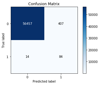
let’s see what variables are more important to the model in absolute value. In the chart below you can see the top 15 most relevant features:
 #calculate the weights
 weights = lr.params
#creates a dataframe for them and the coefficient names importance_list = pd.DataFrame( {'names': features, 'weights': weights })
#normalized absolute weights
 importance_list['abs_weights'] = np.abs(importance_list['weights'])
 total = sum(importance_list['abs_weights'])
 importance_list['norm_weights'] = importance_list['abs_weights']/total
#select top 10 with higher importance
 importance_list = importance_list.sort_values(by='norm_weights', ascending=False)
 importance_list = importance_list.iloc[0:14]
#plot them tcharam!
 ax = importance_list['norm_weights'].plot(kind='bar', title ="Variable importance",figsize=(15,10),legend=True, fontsize=12)
 ax.set_xticklabels(importance_list['names'], rotation=90)
plt.show() 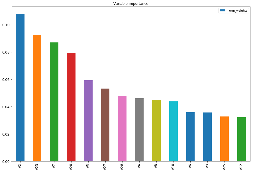
Now to visualize the weights we can see in the plot below which variables decrease x increase the likelihood of having a fradulent transaction.
ax = importance_list['weights'].plot(kind='bar', title ="Variable importance",figsize=(15,10),legend=True, fontsize=12) ax.set_xticklabels(importance_list['names'], rotation=90) plt.show() 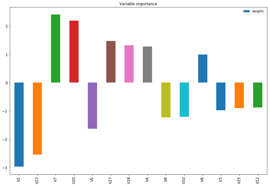
I know this is a pretty long tutorial but hopefully you will not need to go through all the yak shaving I had to go through what I went through.